Expectation Propagation for Probabilistic Bipartite Matching

Given two sets of objects and a matrix of probabilities for matching them, how can we approximate the matching marginals?

In this post I sketch an iterative algorithm for probabilistic bipartite matching. A weighted bipartite matching instance consists of a bipartite graph with a weight associated to each edge. A valid matching assigns exactly one vertex from one partition to one in the other partition. In a probabilistic setting, the weights are log-probabilities, and we do not ask for the maximum matching, but for the distribution of matchings.

More specifically, we denote the partitions by \(V, W\) with vertices \(v_i, i = 1,\ldots, N\) and \(w_j, j = 1,\ldots,M\). The edges are represented by a matrix of potentials \(\mu\), and the matching variable by \(z\), with \(z_{ij} = 1\) if \((v_i, w_j)\) is in the matching. For now, we focus on perfect matchings \(M = N\) and all vertices matched. The corresponding constraints are

\[\begin{align} \sum_j z_{ij} &= 1 &\text{Rows sum to one}\\ \sum_i z_{ij} &= 1 &\text{Columns sum to one} \end{align}\]

Denote the indicator functions for the row (column) constraints by \(f_r(z)\) and \(f_c(z)\), respectively, i.e.

\[f_r(z) = \prod_i \left[\sum_j z_{ij} = 1\right]\]

Then the probability is

\[p(z) = \frac{1}{Z} \underbrace{e^{\sum_{ij}\mu_{ij} z_{ij}}}_{\equiv f_0(z)} \,f_r(z) f_c(z)\]

where \(Z\) is the partition function. Evaluating the partition function is in #P in general, but there are tractable partial problems that allow for efficient simplification.

Namely, if \(f_c(z)\) is dropped we are left with independent Bernoullis with a sum-to-one constraint on the rows - i.e. just a bunch of independent categorical variables. The same holds for dropping \(f_r(z)\). This measure factorization allows to apply Expectation Propagation (EP) to this problem.

Recall that in EP each factor \(f_i(z)\) is approximated by a simpler approximation \(g_i(z)\). Here we approximate all factors by independent Bernoulli distributions, i.e.

\[\begin{align} g_r(z) &= \prod_i g_{r,i}(z) \\ &= \prod_i C_{r,i} \, e^{\sum_j \nu_{r,ij} z_{ij}} \end{align}\]

The factor \(f_0(z)\) is already tractable and need not be approximated.

The approximate posterior is

\[\begin{align} q(z) &\propto f_0(z) g_r(z) g_c(z) \end{align}\]

Expectation Propagation: The Basic Building Block

The EP algorithm consists of iteratively refining the factor approximations by matching the zeroth and first moments. Since each factor involves a sum-to-one constraint, we consider the update for this kind of factor.

The target distribution is characterized by

\[Z(\phi) = \sum_z \left[\sum_i z_i = 1 \right] \, e^{\sum_i \phi_i z_i},\]

and we want to approximate it with

\[Y(\phi; \nu, C) = C \sum_z e^{\sum_i \left(\phi_i + \nu_i\right) z_i}\]

The parameters \(\nu, C\) are set such that the moments

\[\begin{align} Z(\phi) &= \sum_i e^{\phi_i} \\ \pi_i &\equiv \partial_{\phi_i} \log Z(\phi) \\ &= \frac{e^{\phi_i}}{Z(\phi)} \end{align}\]

match those of \(Y(\phi; \nu, C)\). From elementary calculations we get

\[\begin{align} \nu_i &= \log\frac{\pi_i}{1 - \pi_i} - \phi_i \\ C &= \frac{Z(\phi)}{\prod_i \left(1 + e^{\phi_i + \nu_i}\right)} \end{align}\]

Note that \(C\) does not show up as an input to other calculations. It can be evaluated at the end of the iteration or omitted entirely.

Putting it together

In order to do the full problem, all we need to do is pick out a row or column and apply the basic building block recipe. We keep track of the natural parameters \(\nu_{r,ij}, \nu_{c,ij}\) and update them one factor at a time until convergence. Afterwards, we compute the constants \(C_{r,i}\) and \(C_{c, j}\) once.

To update e.g. the constraint on the \(i\)-th row, we use

\[\phi_j = \mu_{ij} + \nu_{c,ij}\]

as background potential. All columns (rows) can be updated in parallel since the constraints do not have overlapping variables.

Limiting Cases

Let’s do a check on a solvable special case in order to get intuition. We consider \(\mu_{ij} = 0\), so that all configurations have the same probability. Clearly, the marginals are just \(\pi_{ij} = \frac{1}{N}\) by symmetry. Similarly, since all rows and columns are symmetric, we obtain a single approximate potential \(\nu\) for all of them. The update equation for the marginals yields

\[\nu = \log\frac{1}{N - 1} - \nu\]

The \(\nu\) on the RHS originates in the fact that each cell is affected by two constraints. The solution is

\[2\nu = \log\frac{1}{N - 1}\]

so that the approximate marginals are

\[\frac{1}{1 + e^{-2\nu}} = \frac{1}{N}\]

A more interesting question is how well the partition function is approximated.

Since each configuration has unit weight, and there are \(N!\) possibilities for matching, we get

\[Z = N!\]

From the basic update above and the marginals we obtain a factor

\[C = \frac{N e^\nu}{\left(1 + e^{2\nu}\right)^N}\]

for each column and row, i.e. \(2N\) in total. This is combined with the normalization of the Bernoulli approximation to obtain the partition function. Here is how it compares to the exact solution:

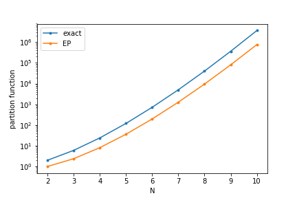
While this is not spectacularly good, the approximation captures the dependence on \(N\). Moreover, this is the worst case for the approximation with independent Bernoullis. If we consider the opposite limit of probabilities that all \(\mu_{ij} = \pm \infty\) and such that they specify a valid solution (i.e. respecting all sum constraints), then the approximation is exact.

In practice, we are somewhere in the middle. Based on the above considerations, we can expect the approximation to be better the closer the probabilities are to specifying a unique solution.

Extensions

It is straightforward to extend the algorithm to more general situations. In particular, constraints of the forms

\[\begin{align} f(z) &= \left[ \sum_i z_i \leq 1 \right] & \text{Optional match} \\ f(z) &= \left[ \sum_i z_i \geq 1 \right] & \text{Allow multiple matches} \end{align}\]

can be dealt with in the same way since the required moments can be evaluated in closed form.

I explain how to compute the moments for more general sum constraints here

Expectation Propagation: The Basic Building Block

Putting it together

Limiting Cases

Extensions

Links