Approximate Conditionally Conjugate Prior for the 2d von Mises-Fisher Distribution
The von Mises-Fisher (vMF) distribution is the analogue of a spherically symmetric Gaussian on the sphere. It is characterized by a mean parameter and a scalar precision. In contrast to the Gaussian, it only has a conjugate prior for the mean parameter (the vMF distribution), but not for the precision due to its normalizer.
In this post I deal with the vMF distribution for the two-sphere and describe a simple approximation that allows for a conjugate prior on the precision, provided the precision is reasonably large. This is useful in Bayesian inference, e.g. for clustering points on the surface of the earth.
von Mises-Fisher Distribution
The vMF distribution for a unit vector \(\mathbf{x}\) is given by
\[\text{vMF}(\mathbf{x} \mid \mathbf{m},\kappa) = \underbrace{\frac{1}{4\pi}}_{\text{base measure}} \underbrace{\frac{\kappa}{\sinh{\kappa}}}_{Z^{-1}(\kappa)} e^{\kappa \mathbf{m}\cdot\mathbf{x}}\]where \(\mathbf{m}\) is a unit vector that parametrizes the mean, and \(\kappa\) is the precision. The base measure is just the inverse area of the unit sphere. The sufficient statistics for observations \(\mathbf{X}\) with \(i\)-th observation \(\mathbf{x}_i\) are given by
\[\mathbf{s} = \sum_{i=1}^n \mathbf{x}_i.\]We can use the analogy to the normal distribution to motivate looking for a prior of the form
\[p(\mathbf{m}, \kappa) = \underbrace{\text{vMF}(\mathbf{m}, \mathbf{r}_0, \kappa)}_{p(\mathbf{m} \mid \kappa)}\,p(\kappa).\]However, since the sphere is compact, we can alternatively use a flat prior \(p(\mathbf{m}) = \frac{1}{4\pi}\) for the mean parameter as well.
In order to infer \(\kappa\) for some observations summarized by sufficient statistics \(\mathbf{s}\), we marginalize \(\mathbf{m}\):
\[\begin{align} p(\mathbf{X}, \kappa) &= \int \frac{d\mathbf{m}}{4\pi} \left[\prod_i p(\mathbf{x}_i\mid \mathbf{m}, \kappa)\right] \, p(\mathbf{m} \mid \kappa) \, p(\kappa) \\ &\propto \frac{Z\left(\kappa \sigma \right)}{Z^\nu(\kappa)} p(\kappa) \end{align}\]where
\[\begin{align} \sigma &= \|\mathbf{s} + \mathbf{r}_0\| \\ \nu &= n + k \end{align}\]and we set \(k = 0, \mathbf{r}_0 = 0\) for the flat prior, while \(k = 1\) for the vMF prior with finite precision.
Approximation for Moderately Large \(\kappa\)
The presence of the \(\sinh\kappa\) term in the normalizer prevents finding a nice conjugate prior, so let’s see whether we can approximate it. Luckily, a reasonable approximation can be obtained directly from the defintion of the sinh,
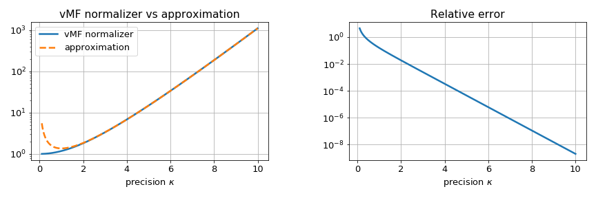
\[\begin{align} \sinh x &= \frac{1}{2} \left(e^x - e^{-x}\right) \\ &\overset{x\gg 1}{\approx} \frac{e^x}{2} \end{align}\]Since the relative error decreases like \(e^{-2\kappa}\), the approximation improves rapidly with increasing \(\kappa\):

While this looks good, it has to be noted that in the posterior the precision is multiplied by \(\|\mathbf{s} + \mathbf{r}_0\|\), so that it can be arbitrarily small! The point is that the approximation works out if the posterior precision is large, not just the prior. In practice, however, the conditions are often met in geospatial applications, where even \(\kappa = 10\) implies an expected radius of around \(3{,}000\text{km}\) (or \(3\text{Mm}\) for SI purists) and covers roughly the area of North America. At \(\kappa = 2.5\), close to where the approximation starts to break down, it covers an area of the size of the Atlantic - or more than 20% of the earth’s surface.
The advantage gained is that the normalizer has the form \(\kappa^a e^{-b \kappa}\), so that the Gamma distribution can be used as a conjugate prior for \(\kappa\). In fact,
\[\begin{align} \frac{Z(\sigma \kappa)}{Z^\nu(\kappa)} \text{Gamma}(\kappa \mid \alpha, \beta) &\overset{\kappa\gg 1}{\propto} \kappa^{\alpha - 1 + \nu - 1} e^{-\left(\beta + \nu - \sigma\right)\kappa} \\ &\propto \text{Gamma}\left(\alpha + \nu - 1, \beta + \nu - \sigma\right), \end{align}\]Let’s have a look at the behavior of the posterior. The posterior mean of \(\kappa\) is
\[\mathbb{E}[\kappa] = \frac{\alpha + \nu - 1}{\beta + \nu - \sigma}\]Since \(\sigma\) is the length of a sum of unit vectors, \(0\leq \sigma \leq \nu\), so that the posterior mean satisfies
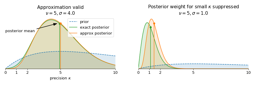
\[\frac{\alpha + \nu - 1}{\beta + \nu} \leq \mathbb{E}[\kappa] \leq \frac{\alpha + \nu - 1}{\beta}\]The lower bound corresponds to \(\sigma = 0\) and tends to one as \(\nu\rightarrow\infty\). Without approximations, it the posterior mean approaches zero. This is to be expected, since the approximate partition function diverges around \(\kappa = 0\) instead of approaching a constant value. This behavior is illustrated here:

Summary
In summary, I have shown how to derive an approximation to the normalizer of the von Mises-Fisher distribution that allows conditionally conjugate computations similar to the Normal distribution. I think the combination of simplicity and applicability to a wide range of parameters make this useful in particular for Bayesian clustering / mixtures, where it allows to collapse both cluster parameters in closed form instead of just the mean.